Timoshenko Beam
#

elastica.modules用于构建不同的仿真系统

import numpy as np

# Import modules
from elastica.modules import BaseSystemCollection, Constraints, Forcing, Damping

# Import Cosserat Rod Class
from elastica.rod.cosserat_rod import CosseratRod

# Import Damping Class
from elastica.dissipation import AnalyticalLinearDamper

# Import Boundary Condition Classes
from elastica.boundary_conditions import OneEndFixedRod, FreeRod
from elastica.external_forces import EndpointForces

# Import Timestepping Functions
from elastica.timestepper.symplectic_steppers import PositionVerlet
from elastica.timestepper import integrate

在这个例子中，杆的一端被固定住，令另一端受力。

class TimoshenkoBeamSimulator(BaseSystemCollection, Constraints, Forcing, Damping):
    pass


timoshenko_sim = TimoshenkoBeamSimulator()

接下来，定义这个杆的各项属性，包括材料、几何形状等。

# setting up test params
# rod 中单元体 elements 的数量
n_elem = 100

density = 1000
nu = 1e-4
E = 1e6  # 弹性模量
# For shear modulus of 1e4, nu is 99!
# 泊松比，一般不超过0.5，这里是为了让变形更明显
poisson_ratio = 99 
shear_modulus = E / (poisson_ratio + 1.0) # 剪切系数

# 三维空间中的起始坐标
start = np.zeros((3,))
# rod 的朝向
direction = np.array([0.0, 0.0, 1.0])
normal = np.array([0.0, 1.0, 0.0])
base_length = 3.0
base_radius = 0.25
base_area = np.pi * base_radius ** 2

我们根据上述的参数构建出一根 rod，然后把它加入到一开始创建的仿真系统中

shearable_rod = CosseratRod.straight_rod(
    n_elem,
    start,
    direction,
    normal,
    base_length,
    base_radius,
    density,
    0.0,     # internal damping constant, deprecated in v0.3.0
    E,
    shear_modulus=shear_modulus,
)

timoshenko_sim.append(shearable_rod)

添加阻尼
#

We also need to define damping_constant and simulation time_step and pass in .using() method.

dl = base_length / n_elem
dt = 0.01 * dl
timoshenko_sim.dampen(shearable_rod).using(
    AnalyticalLinearDamper,
    damping_constant=nu,
    time_step=dt,
)

添加边界条件
#

第一个约束是，固定杆一端的位置。We do this using the .constrain()option and theOneEndFixedRodboundary condition. We are modifying thetimoshenko_simsimulator toconstraintheshearable_rodobject using theOneEndFixedRod type of constraint.

我们还要定义杆的哪一个节点需要被约束.，可以通过节点的索引 constrained_position_idx来实现，这里我们固定了第一个节点。为了防止杆绕固定节点旋转, 我们需要在两个节点之间约束一个元素，这固定了杆的方向. 我们通过约束元素的索引 constrained_director_idx来实现。例如对于 position, 我们约束杆的第一个元素. Together, this contrains the position and orientation of the rod at the origin.

timoshenko_sim.constrain(shearable_rod).using(
    OneEndFixedRod, constrained_position_idx=(0,), constrained_director_idx=(0,)
)
print("One end of the rod is now fixed in place")

第二个约束是对杆的末端施加一个力。我们想在d1方向施加一个负的力，同时加到杆的末端，可以通过指定origin_force 和end_force 实现。我们还想随着时间逐渐提高力的大小，通过指定ramp_up_time来改变，这防止了因力的不连续导致的错误。

origin_force = np.array([0.0, 0.0, 0.0])
end_force = np.array([-10.0, 0.0, 0.0])
ramp_up_time = 5.0

timoshenko_sim.add_forcing_to(shearable_rod).using(
    EndpointForces, origin_force, end_force, ramp_up_time=ramp_up_time
)
print("Forces added to the rod")

添加 Unshearable Rod
#

为了比较 shearable rod 和 unshearable rod，我们再添加一个unshearable rod。我们改变 rod 的泊松比来让它 unshearable。对于真实的unshearable rod，泊松比通常为 -1.0，然而这会导致系统数值不稳定，所以我们采用 -0.85 的泊松比。

# Start into the plane
unshearable_start = np.array([0.0, -1.0, 0.0])
unshearable_rod = CosseratRod.straight_rod(
    n_elem,
    unshearable_start,
    direction,
    normal,
    base_length,
    base_radius,
    density,
    0.0,     # internal damping constant, deprecated in v0.3.0
    E,
    # Unshearable rod needs G -> inf, which is achievable with a poisson ratio of -1.0
    shear_modulus=E / (-0.85 + 1.0),
)

timoshenko_sim.append(unshearable_rod)

timoshenko_sim.dampen(unshearable_rod).using(
    AnalyticalLinearDamper,
    damping_constant=nu,
    time_step=dt,
)

timoshenko_sim.constrain(unshearable_rod).using(
    OneEndFixedRod, constrained_position_idx=(0,), constrained_director_idx=(0,)
)

timoshenko_sim.add_forcing_to(unshearable_rod).using(
    EndpointForces, origin_force, end_force, ramp_up_time=ramp_up_time
)
print("Unshearable rod set up")

系统结束
#

现在我们以及添加完需要的rods及其边界条件到我们的系统中。最后，我们需要结束这个系统。这个操作将遍历系统，重新排列事物，并预计算有用的数值，为系统进行仿真做好准备。

timoshenko_sim.finalize()
print("System finalized")

注意，如果在 finalize 后对 rod 做出了一些改变，需要 re-setup 该系统，即重新运行上述的所有代码。

定义仿真时间
#

我们还要决定该仿真的运行时间，以及使用哪种时间步长方法。默认方法是 PositionVerlet 算法。这里我们仿真10s。

final_time = 10.0
total_steps = int(final_time / dt)
print("Total steps to take", total_steps)

timestepper = PositionVerlet()

运行仿真
#

对于仿真的运行，我们结合 timoshenko_sim，使用 timestepper 方法，执行了 total_steps 步后，到达 final_time。

integrate(timestepper, timoshenko_sim, final_time, total_steps)

‍

Post Processing Results
#

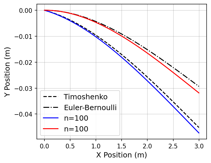
现在仿真已经结束，我们想处理仿真结果，我们将比较the solutions for the shearable and unshearable beams与analytical Timoshenko and Euler-Bernoulli beam results.

# Compute beam position for sherable and unsherable beams.
def analytical_result(arg_rod, arg_end_force, shearing=True, n_elem=500):
    base_length = np.sum(arg_rod.rest_lengths)
    # 在间隔 0.0 和 base_length 之间返回 n_elem 个均匀间隔的数据
    # 即每个节点距离起始点的长度
    arg_s = np.linspace(0.0, base_length, n_elem)
    if type(arg_end_force) is np.ndarray:
        acting_force = arg_end_force[np.nonzero(arg_end_force)]
    else:
        acting_force = arg_end_force
    acting_force = np.abs(acting_force)
    linear_prefactor = -acting_force / arg_rod.shear_matrix[0, 0, 0]
    quadratic_prefactor = (
        -acting_force
        / 2.0
        * np.sum(arg_rod.rest_lengths / arg_rod.bend_matrix[0, 0, 0])
    )
    cubic_prefactor = (acting_force / 6.0) / arg_rod.bend_matrix[0, 0, 0]
    if shearing:
        return (
            arg_s,
            arg_s * linear_prefactor
            + arg_s ** 2 * quadratic_prefactor
            + arg_s ** 3 * cubic_prefactor,
        )
    else:
        return arg_s, arg_s ** 2 * quadratic_prefactor + arg_s ** 3 * cubic_prefactor

现在，我们想去画出结果。首先需要指出的是，如何接收杆的位置，它们位于rod.position_collection[dim, n_elem]。在本例中，我们画出 x- 和 z-轴。

def plot_timoshenko(shearable_rod, unshearable_rod, end_force):
    import matplotlib.pyplot as plt

    analytical_shearable_positon = analytical_result(
        shearable_rod, end_force, shearing=True
    )
    analytical_unshearable_positon = analytical_result(
        unshearable_rod, end_force, shearing=False
    )

    fig = plt.figure(figsize=(5, 4), frameon=True, dpi=150)
    ax = fig.add_subplot(111)
    ax.grid(b=True, which="major", color="grey", linestyle="-", linewidth=0.25)

    ax.plot(
        analytical_shearable_positon[0],
        analytical_shearable_positon[1],
        "k--",
        label="Timoshenko",
    )
    ax.plot(
        analytical_unshearable_positon[0],
        analytical_unshearable_positon[1],
        "k-.",
        label="Euler-Bernoulli",
    )

    ax.plot(
        shearable_rod.position_collection[2, :],
        shearable_rod.position_collection[0, :],
        "b-",
        label="n=" + str(shearable_rod.n_elems),
    )
    ax.plot(
        unshearable_rod.position_collection[2, :],
        unshearable_rod.position_collection[0, :],
        "r-",
        label="n=" + str(unshearable_rod.n_elems),
    )

    ax.legend(prop={"size": 12})
    ax.set_ylabel("Y Position (m)", fontsize=12)
    ax.set_xlabel("X Position (m)", fontsize=12)
    plt.show()


plot_timoshenko(shearable_rod, unshearable_rod, end_force)

‍

Timoshenko Beam #

添加阻尼 #

添加边界条件 #

添加 Unshearable Rod #

系统结束 #

定义仿真时间 #

运行仿真 #

Post Processing Results #